PLSLDA - breast dataset#
[1]:
#disable warnings
from warnings import simplefilter, filterwarnings
simplefilter(action='ignore', category=FutureWarning)
filterwarnings("ignore")
breast dataset#
[2]:
#alcools dataset
from discrimintools.datasets import load_dataset
D = load_dataset("breast")
D.info()
<class 'pandas.core.frame.DataFrame'>
RangeIndex: 699 entries, 0 to 698
Data columns (total 4 columns):
 #   Column     Non-Null Count  Dtype
---  ------     --------------  -----
 0   ucellsize  699 non-null    int64
 1   normnucl   699 non-null    int64
 2   mitoses    699 non-null    int64
 3   Class      699 non-null    object
dtypes: int64(3), object(1)
memory usage: 22.0+ KB
[3]:
#split into X and y
y, X = D["Class"], D.drop(columns=["Class"])
Instanciation and training#
[4]:
#instanciation and training
from discrimintools import PLSLDA
clf = PLSLDA()
clf.fit(X,y)
[4]:
PLSLDA()In a Jupyter environment, please rerun this cell to show the HTML representation or trust the notebook.
On GitHub, the HTML representation is unable to render, please try loading this page with nbviewer.org.
Parameters
| n_components | 2 | |
| scale | True | |
| priors | None | |
| classes | None | |
| max_iter | 500 | |
| tol | 1e-10 | |
| var_select | False | |
| threshold | 1.0 | |
| warn_message | True |
Canonical coefficients#
[5]:
#canonical coefficients
cancoef = clf.cancoef_
cancoef._fields
[5]:
('standardized', 'raw')
Standardized canonical coefficients#
[6]:
#standardized canonical coefficients
print(cancoef.standardized)
               Can1      Can2
ucellsize  0.702554 -0.605737
normnucl   0.611795  0.025466
mitoses    0.363490  0.803929
Raw canonical coefficients#
[7]:
#raw canonical coefficients
print(cancoef.raw)
               Can1      Can2
Constant  -1.632918 -0.146717
ucellsize  0.230235 -0.198507
normnucl   0.200350  0.008340
mitoses    0.211938  0.468742
Coefficients#
[8]:
#coefficients
coef = clf.coef_
coef._fields
[8]:
('standardized', 'raw')
Standardized coefficients#
[9]:
#standardized coefficients
print(coef.standardized)
           negative  positive
Constant  -1.022831 -3.231980
ucellsize -1.302482  2.475256
normnucl  -0.813468  1.545927
mitoses   -0.025749  0.048934
Raw coefficients#
[10]:
#raw coefficients
print(coef.raw)
           negative  positive
Constant   1.102686 -7.271345
ucellsize -0.426839  0.811171
normnucl  -0.266394  0.506258
mitoses   -0.015013  0.028531
Summary#
[11]:
#summary
from discrimintools import summaryPLSLDA
summaryPLSLDA(clf,detailed=True)
                     Partial Least Squares Linear Discriminant Analysis - Results

Class Level Information:
          Frequency  Proportion  Prior Probability
negative        458      0.6552             0.6552
positive        241      0.3448             0.3448

Importance of PLS components:
      Proportion (%)  Cumulative (%)
Can1         69.1520         69.1520
Can2         20.1981         89.3501

Raw Canonical and Classification Functions Coefficients:
             Can1    Can2  negative  positive
Constant  -1.6329 -0.1467    1.1027   -7.2713
ucellsize  0.2302 -0.1985   -0.4268    0.8112
normnucl   0.2003  0.0083   -0.2664    0.5063
mitoses    0.2119  0.4687   -0.0150    0.0285

Multivariate Analysis of Variance (MANOVA) Summary:
          Statistic     Value  p-value
0     Wilks' Lambda    0.3042      NaN
1  Bartlett -- C(2)  828.2718      0.0
2   Rao -- F(2,696)  795.9566      0.0

LDA Classification functions & Statistical Evaluation:
          negative  positive  Wilks' Lambda  Partial R-Square    F Value  \
Constant   -1.0228   -3.2320            NaN               NaN        NaN
Can1       -1.3538    2.5728         0.9666            0.3147  1515.4447
Can2        0.5801   -1.1024         0.3376            0.9010    76.4684

          Num DF  Den DF  Pr>F
Constant     NaN     NaN   NaN
Can1         1.0   696.0   0.0
Can2         1.0   696.0   0.0

Classification Summary for Calibration Data:

Observation Profile:
                        Read  Used
Number of Observations   699   699

Number of Observations Classified into Class:
prediction  negative  positive  Total
Class
negative         447        11    458
positive          55       186    241
Total            502       197    699

Percent Classified into Class:
prediction  negative  positive  Total
Class
negative     97.5983    2.4017  100.0
positive     22.8216   77.1784  100.0
Total        71.8169   28.1831  100.0
Priors        0.6552    0.3448    NaN

Error Count Estimates for Class:
        negative  positive   Total
Rate      0.0240    0.2282  0.0944
Priors    0.6552    0.3448     NaN

Classification Report for Class:
              precision  recall  f1-score   support
negative         0.8904  0.9760    0.9312  458.0000
positive         0.9442  0.7718    0.8493  241.0000
accuracy         0.9056  0.9056    0.9056    0.9056
macro avg        0.9173  0.8739    0.8903  699.0000
weighted avg     0.9090  0.9056    0.9030  699.0000
Plotting#
[12]:
#plotting
from discrimintools import fviz_plsr
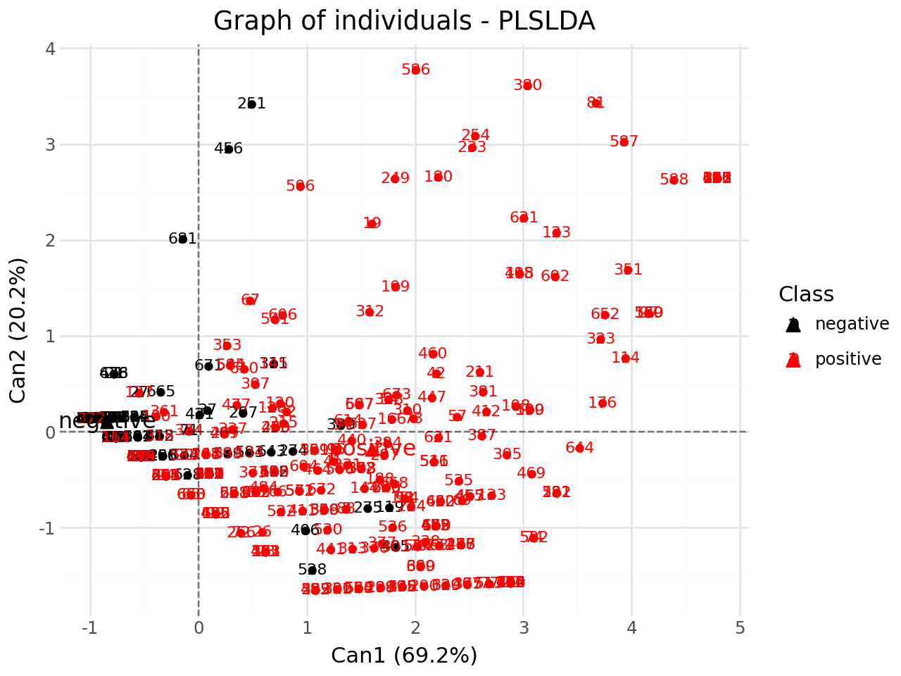
Graph of individuals#
[13]:
#graph of individuals
p = fviz_plsr(clf,element="ind",repel=False)
p.show()
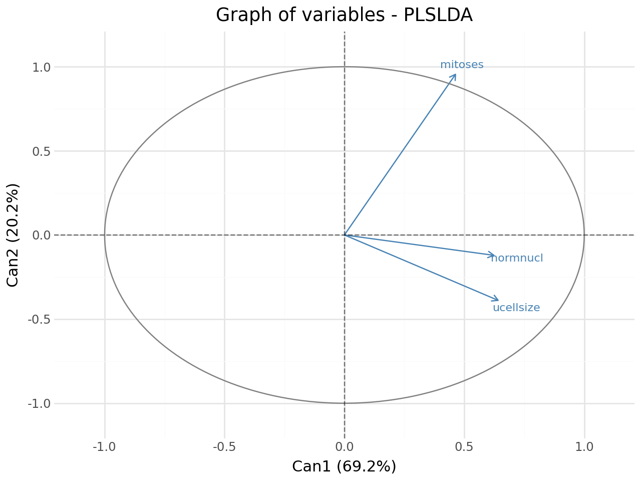
Graph of variables#
[14]:
#graph of variables
p = fviz_plsr(clf,element="var",repel=True)
p.show()
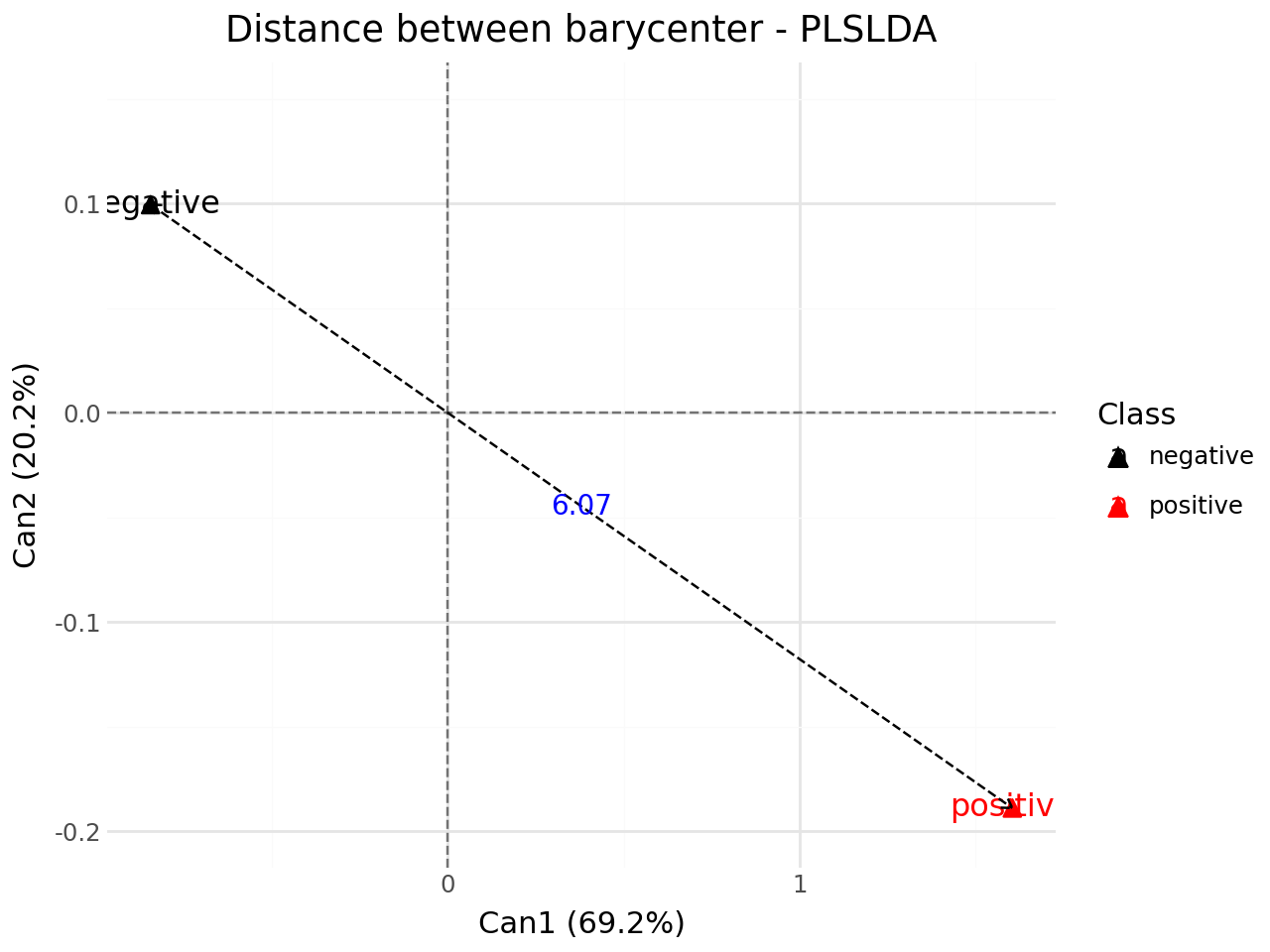
Distance between barycenter#
[15]:
#distance between barycenter
p = fviz_plsr(clf,element="dist",repel=False,y_lim=(-0.2,0.15))
p.show()