CANDISC - vins dataset#
[1]:
#disable warnings
from warnings import simplefilter, filterwarnings
simplefilter(action='ignore', category=FutureWarning)
filterwarnings("ignore")
vins dataset#
[2]:
#vins dataset
from discrimintools.datasets import load_vins
D = load_vins()
print(D.info())
<class 'pandas.core.frame.DataFrame'>
Index: 34 entries, 1924 to 1957
Data columns (total 5 columns):
 #   Column       Non-Null Count  Dtype
---  ------       --------------  -----
 0   Temperature  34 non-null     int64
 1   Soleil       34 non-null     int64
 2   Chaleur      34 non-null     int64
 3   Pluie        34 non-null     int64
 4   Qualite      34 non-null     object
dtypes: int64(4), object(1)
memory usage: 1.6+ KB
None
[3]:
#split into X and y
y, X = D["Qualite"], D.drop(columns=["Qualite"])
instanciation & training#
[4]:
from discrimintools import CANDISC
clf = CANDISC(n_components=2,classes=("Mediocre","Moyen","Bon"))
fit function#
[5]:
#fit function
clf.fit(X,y)
[5]:
CANDISC(classes=('Mediocre', 'Moyen', 'Bon'))
In a Jupyter environment, please rerun this cell to show the HTML representation or trust the notebook. On GitHub, the HTML representation is unable to render, please try loading this page with nbviewer.org.
Parameters
| n_components | 2 | |
| classes | ('Mediocre', ...) | |
| warn_message | True |
eval_predict function#
[6]:
#eval_predict function
eval_train = clf.eval_predict(X,y,verbose=True)
Observation Profile:
                        Read  Used
Number of Observations    34    34

Number of Observations Classified into Qualite:
prediction  Mediocre  Moyen  Bon  Total
Qualite
Mediocre          10      2    0     12
Moyen              1      8    2     11
Bon                0      2    9     11
Total             11     12   11     34

Percent Classified into Qualite:
prediction   Mediocre      Moyen        Bon  Total
Qualite
Mediocre    83.333333  16.666667   0.000000  100.0
Moyen        9.090909  72.727273  18.181818  100.0
Bon          0.000000  18.181818  81.818182  100.0
Total       32.352941  35.294118  32.352941  100.0
Priors       0.352941   0.323529   0.323529    NaN

Error Count Estimates for Qualite:
        Mediocre     Moyen       Bon     Total
Rate    0.166667  0.272727  0.181818  0.205882
Priors  0.352941  0.323529  0.323529       NaN

Classification Report for Qualite:
              precision    recall  f1-score    support
Mediocre       0.909091  0.833333  0.869565  12.000000
Moyen          0.666667  0.727273  0.695652  11.000000
Bon            0.818182  0.818182  0.818182  11.000000
accuracy       0.794118  0.794118  0.794118   0.794118
macro avg      0.797980  0.792929  0.794466  34.000000
weighted avg   0.801248  0.794118  0.796675  34.000000
[7]:
#score function
print("Accuracy : {}%".format(100*round(clf.score(X,y),2)))
Accuracy : 79.0%
[8]:
#error rate
print("Error rate : {}%".format(100-100*round(clf.score(X,y),2)))
Error rate : 21.0%
Canonical coefficients#
[9]:
#canonical coefficients
cancoef = clf.cancoef_
cancoef._fields
[9]:
('raw', 'total', 'pooled')
Total Sample Standardized Canonical Coefficients#
[10]:
#Total Sample Standardized Canonical Coefficients
print(cancoef.total)
                 Can1      Can2
Temperature  1.209391 -0.006530
Soleil       0.857727 -0.674811
Chaleur     -0.270993  1.278476
Pluie       -0.536131  0.564364
Pooled Within class Standardized Canonical Coefficients#
[11]:
#Pooled Within class Standardized Canonical Coefficients
print(cancoef.pooled)
                 Can1      Can2
Temperature  0.750126 -0.004050
Soleil       0.547064 -0.430399
Chaleur     -0.198237  0.935229
Pluie       -0.445097  0.468536
Raw canonical coefficients#
[12]:
#raw canonical coefficients
print(cancoef.raw)
                  Can1      Can2
Constant    -32.876282  2.165279
Temperature   0.008566 -0.000046
Soleil        0.006774 -0.005329
Chaleur      -0.027054  0.127636
Pluie        -0.005866  0.006175
Class Means on Canonical Variables#
[13]:
#Class Means on Canonical Variables
print(clf.classes_.coord)
              Can1      Can2
Mediocre -2.079247  0.221184
Moyen     0.146307 -0.513104
Bon       2.121963  0.271812
summary#
[14]:
from discrimintools import summaryCANDISC
Simple summary#
[15]:
#simple summary
summaryCANDISC(clf)
                     Canonical Discriminant Analysis - Results

Summary Information:
               infos  Value                  DF  DF value
0  Total Sample Size     34            DF Total        33
1          Variables      4   DF Within Classes        31
2            Classes      3  DF Between Classes         2

Class Level Information:
          Frequency  Proportion  Prior Probability
Mediocre         12      0.3529             0.3529
Moyen            11      0.3235             0.3235
Bon              11      0.3235             0.3235

Total-Sample Class Means:
              Mediocre      Moyen        Bon
Temperature  3037.3333  3140.9091  3306.3636
Soleil       1126.4167  1262.9091  1363.6364
Chaleur        12.0833    16.4545    28.5455
Pluie         430.3333   339.6364   305.0000

Importance of components:
      Eigenvalue  Difference  Proportion  Cumulative
Can1      3.2789      3.1403     95.9451     95.9451
Can2      0.1386         NaN      4.0549    100.0000

Raw Canonical and Classification Functions Coefficients:
                Can1    Can2  Mediocre   Moyen      Bon
Constant    -32.8763  2.1653   65.6093 -7.1918 -72.5905
Temperature   0.0086 -0.0000   -0.0178  0.0013   0.0182
Soleil        0.0068 -0.0053   -0.0153  0.0037   0.0129
Chaleur      -0.0271  0.1276    0.0845 -0.0694  -0.0227
Pluie        -0.0059  0.0062    0.0136 -0.0040  -0.0108
Detailed summary#
[16]:
#detailed summary
summaryCANDISC(clf,detailed=True)
                     Canonical Discriminant Analysis - Results

Summary Information:
               infos  Value                  DF  DF value
0  Total Sample Size     34            DF Total        33
1          Variables      4   DF Within Classes        31
2            Classes      3  DF Between Classes         2

Class Level Information:
          Frequency  Proportion  Prior Probability
Mediocre         12      0.3529             0.3529
Moyen            11      0.3235             0.3235
Bon              11      0.3235             0.3235

Total-Sample Class Means:
              Mediocre      Moyen        Bon
Temperature  3037.3333  3140.9091  3306.3636
Soleil       1126.4167  1262.9091  1363.6364
Chaleur        12.0833    16.4545    28.5455
Pluie         430.3333   339.6364   305.0000

Importance of components:
      Eigenvalue  Difference  Proportion  Cumulative
Can1      3.2789      3.1403     95.9451     95.9451
Can2      0.1386         NaN      4.0549    100.0000

Raw Canonical and Classification Functions Coefficients:
                Can1    Can2  Mediocre   Moyen      Bon
Constant    -32.8763  2.1653   65.6093 -7.1918 -72.5905
Temperature   0.0086 -0.0000   -0.0178  0.0013   0.0182
Soleil        0.0068 -0.0053   -0.0153  0.0037   0.0129
Chaleur      -0.0271  0.1276    0.0845 -0.0694  -0.0227
Pluie        -0.0059  0.0062    0.0136 -0.0040  -0.0108

Test of H0: The canonical correlations in the current row and all that follow are zero
   Canonical Correlation  Squared Canonical Correlation  Likelihood Ratio  \
0                 0.8754                         0.7663            0.2053
1                 0.3489                         0.1217            0.8783

   Approximate F value  Num DF  Den DF    Pr>F  Chi-Square  DF  Pr>Chi2
0               8.4505       8      56  0.0000     46.7122   8   0.0000
1               1.3395       3      29  0.2808      3.8284   3   0.2806

Classification Summary for Calibration Data:

Observation Profile:
                        Read  Used
Number of Observations    34    34

Number of Observations Classified into Qualite:
prediction  Mediocre  Moyen  Bon  Total
Qualite
Mediocre          10      2    0     12
Moyen              1      8    2     11
Bon                0      2    9     11
Total             11     12   11     34

Percent Classified into Qualite:
prediction  Mediocre    Moyen      Bon  Total
Qualite
Mediocre     83.3333  16.6667   0.0000  100.0
Moyen         9.0909  72.7273  18.1818  100.0
Bon           0.0000  18.1818  81.8182  100.0
Total        32.3529  35.2941  32.3529  100.0
Priors        0.3529   0.3235   0.3235    NaN

Error Count Estimates for Qualite:
        Mediocre   Moyen     Bon   Total
Rate      0.1667  0.2727  0.1818  0.2059
Priors    0.3529  0.3235  0.3235     NaN

Classification Report for Qualite:
              precision  recall  f1-score  support
Mediocre         0.9091  0.8333    0.8696  12.0000
Moyen            0.6667  0.7273    0.6957  11.0000
Bon              0.8182  0.8182    0.8182  11.0000
accuracy         0.7941  0.7941    0.7941   0.7941
macro avg        0.7980  0.7929    0.7945  34.0000
weighted avg     0.8012  0.7941    0.7967  34.0000
Evaluation of prediction on testing dataset#
Testing data#
[17]:
#testining data
XTest = load_vins("test")
print(XTest.info())
<class 'pandas.core.frame.DataFrame'>
Index: 1 entries, 1958 to 1958
Data columns (total 4 columns):
 #   Column       Non-Null Count  Dtype
---  ------       --------------  -----
 0   Temperature  1 non-null      int64
 1   Soleil       1 non-null      int64
 2   Chaleur      1 non-null      int64
 3   Pluie        1 non-null      int64
dtypes: int64(4)
memory usage: 40.0 bytes
None
prediction on testing data#
[18]:
#predict on testing data
print(clf.predict(XTest))
1958    Mediocre
Name: prediction, dtype: object
Coordinates of new individual#
[19]:
#coordinates of new individual
print(clf.transform(XTest))
          Can1      Can2
1958 -2.027679  0.569395
Plotting#
[20]:
#plotting
from discrimintools import fviz_candisc
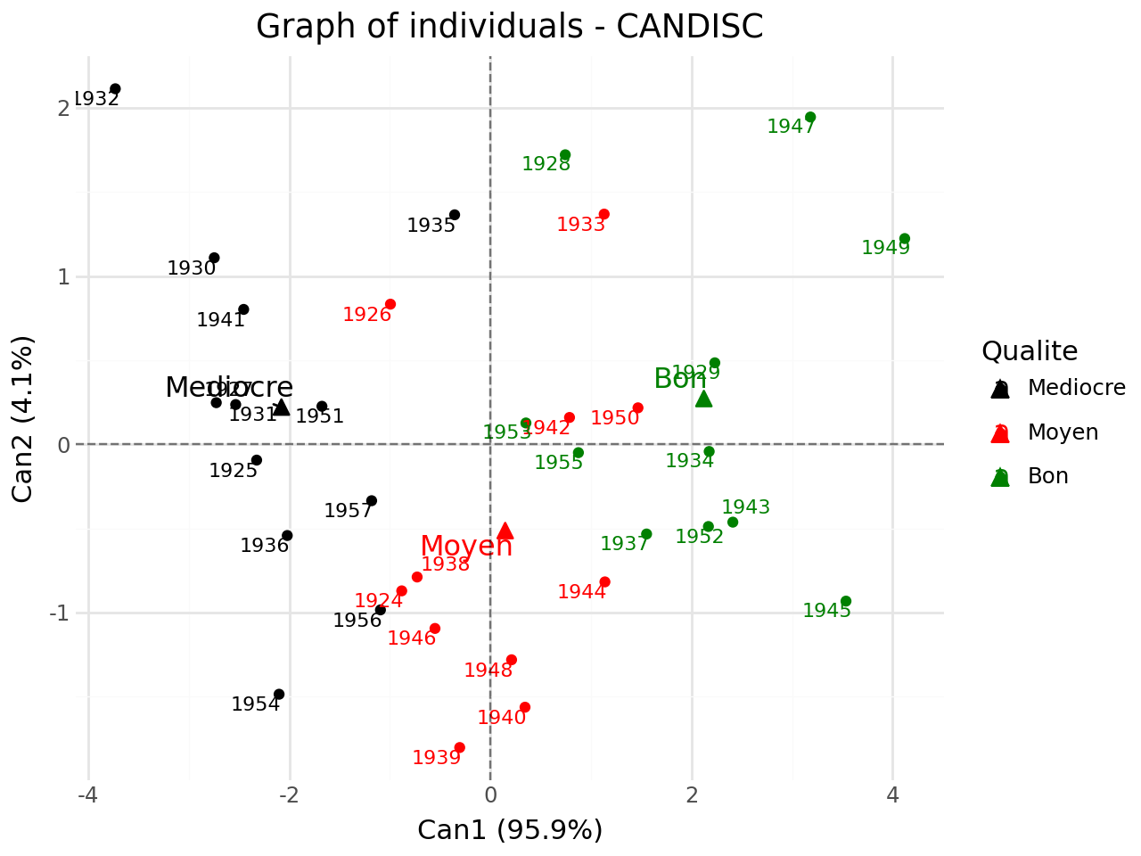
Graph of individuals#
[21]:
#graph of individuals
p = fviz_candisc(clf,element="ind",repel=True)
p.show()
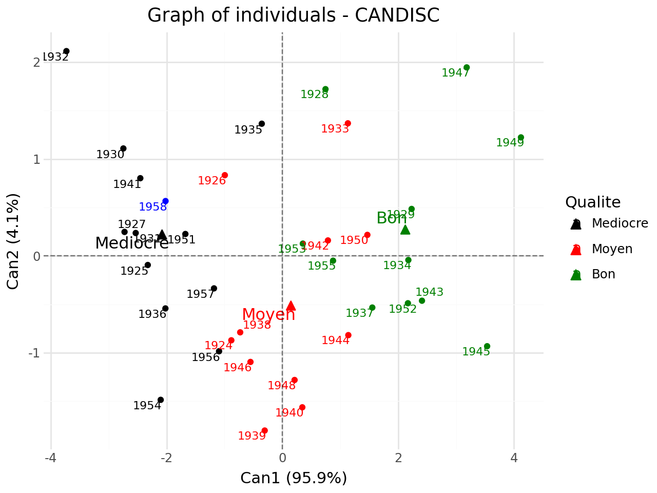
We add supplementary individuals to initial plot.
[22]:
#with supplementary individuals
from discrimintools import add_scatter
p = add_scatter(p,clf.transform(XTest),color="blue",repel=True)
p.show()
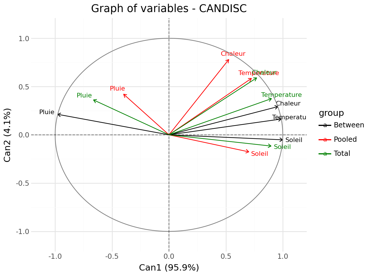
Graph of variables#
[23]:
#graph of variables
fviz_candisc(clf,element="var",repel=True).show()
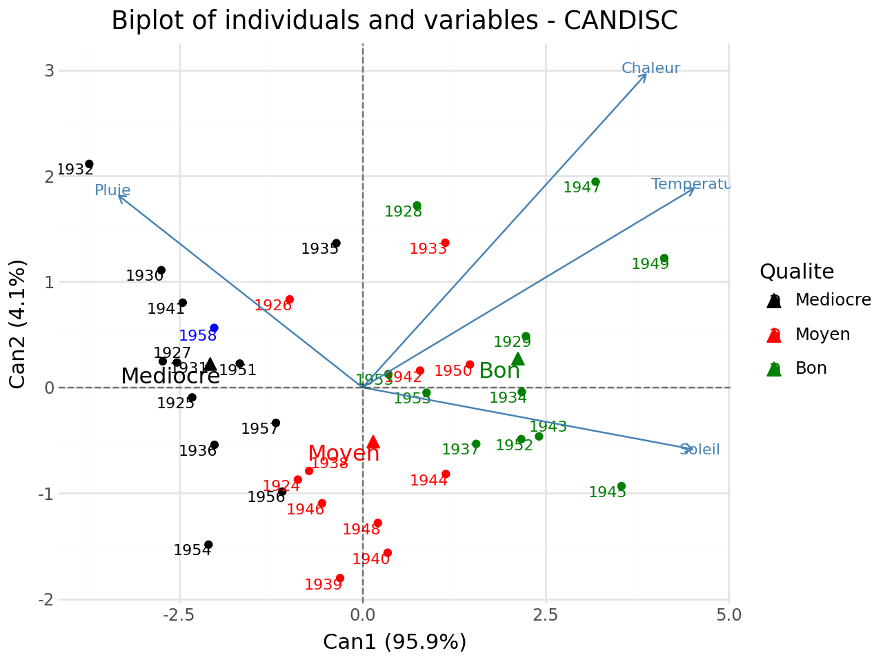
Biplot of individuals and variiables#
[24]:
#biplot of individuals and variables
p = fviz_candisc(clf,element="biplot",repel=True)
#add supplementary individuals
p = add_scatter(p,clf.transform(XTest),color="blue",repel=True)
p.show()
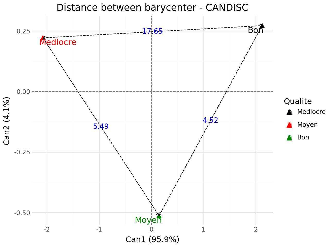
Distance between barycenter#
[25]:
#distance between barycenter
fviz_candisc(clf,element="dist",repel=True).show()